Benchmark Test Functions

For convenience, a collection of benchmark functions is bundled with GloMPO. These may be helpful for testing purposes and may be used to experiment with different configurations and ensure a script is functional before being applied to a more expensive test case.

Ackley	Implementation of the Ackley optimization test function [b].
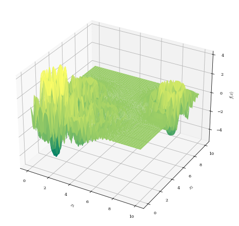
Alpine01	Implementation of the Alpine Type-I optimization test function [a].
Alpine02	Implementation of the Alpine Type-II optimization test function [a].
Deceptive	Implementation of the Deceptive optimization test function [a].
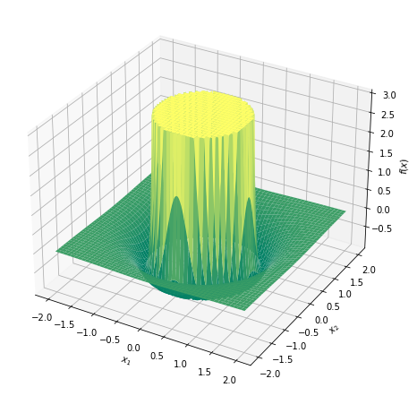
Easom	Implementation of the Easom optimization test function [a].
ExpLeastSquaresCost	Least squares type cost function.
Griewank	Implementation of the Griewank optimization test function [b].
Langermann	When called returns evaluations of the Langermann function [a] [b].
LennardJones	Lennard-Jones energy potential function.
Levy	Implementation of the Levy optimization test function [b].
Michalewicz	Implementation of the Michalewicz optimization test function [b].
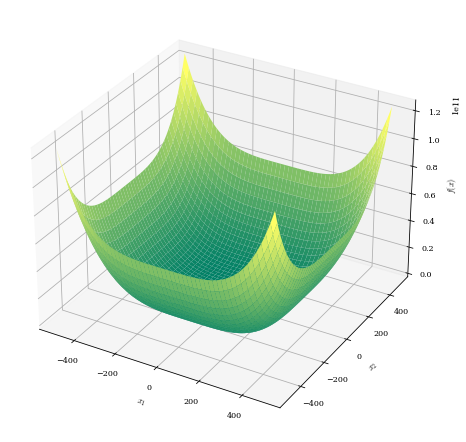
Qing	Implementation of the Qing optimization test function [a].
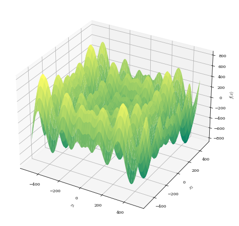
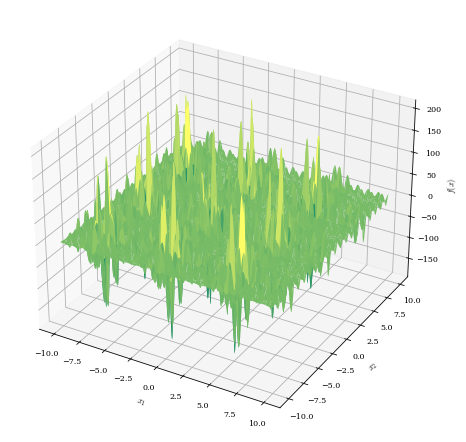
Rana	Implementation of the Rana optimization test function [a].
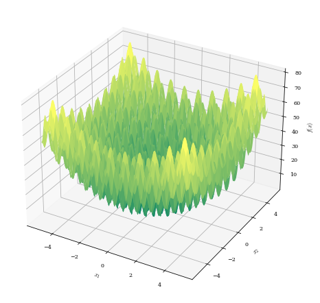
Rastrigin	Implementation of the Rastrigin optimization test function [b].
Rosenbrock	Implementation of the Rosenbrock optimization test function [b].
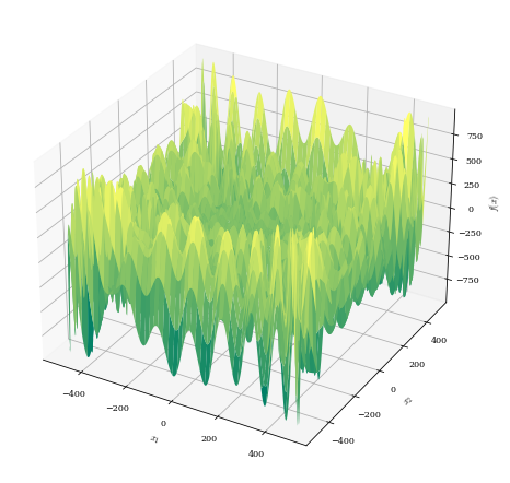
Schwefel	Implementation of the Schwefel optimization test function [b].
Shekel	Implementation of the Shekel optimization test function [b].
Shubert	Implementation of the Shubert Type-I, Type-III and Type-IV optimization test functions [a].
Stochastic	Implementation of the Stochastic optimization test function [a].
StyblinskiTang	Implementation of the Styblinski-Tang optimization test function [b].
Trigonometric	Implementation of the Trigonometric Type-II optimization test function [a].
Vincent	Implementation of the Vincent optimization test function [a].
ZeroSum	Implementation of the ZeroSum optimization test function [a].

class glompo.benchmark_fncs.BaseTestCase(dims: int, *, delay: float = 0)

Basic API for Optimization test cases.

Parameters:

• dims – Number of parameters in the input space.
• delay – Pause (in seconds) between function evaluations to mimic slow functions.

__call__(x: Sequence[float]) → float

Evaluates the function.

Parameters:x – Vector in parameter space where the function will be evaluated. Returns:Function value at x. Return type:float

bounds

Sequence of min/max pairs bounding the function in each dimension.

delay

Delay (in seconds) between function evaluations to mimic slow functions.

dims

Number of parameters in the input space.

min_fx

The function value of the global minimum.

min_x

The location of the global minimum in parameter space.

class glompo.benchmark_fncs.Ackley(dims: int = 2, a: float = 20, b: float = 0.2, c: float = 6.283185307179586, *, delay: float = 0)

Bases: glompo.benchmark_fncs.BaseTestCase

Implementation of the Ackley optimization test function [b].

\[f(x) = - a \exp\left(-b \sqrt{\frac{1}{d}\sum^d_{i=1}x_i^2}\right) - \exp\left(\frac{1}{d}\sum^d_{i=1}\cos\left(cx_i\right)\right) + a + \exp(1)\]

Recommended bounds: \(x_i \in [-32.768, 32.768]\)

Global minimum: \(f(0, 0, ..., 0) = 0\)

Parameters:

• a – Ackley function parameter
• b – Ackley function parameter
• c – Ackley function parameter

class glompo.benchmark_fncs.Alpine01(dims: int, *, delay: float = 0)

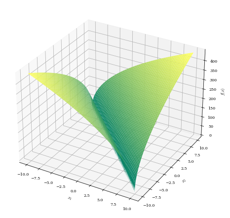
Bases: glompo.benchmark_fncs.BaseTestCase

Implementation of the Alpine Type-I optimization test function [a].

\[f(x) = \sum^n_{i=1}\left|x_i\sin\left(x_i\right)+0.1x_i\right|\]

Recommended bounds: \(x_i \in [-10, 10]\)

Global minimum: \(f(0, 0, ..., 0) = 0\)

class glompo.benchmark_fncs.Alpine02(dims: int, *, delay: float = 0)

Bases: glompo.benchmark_fncs.BaseTestCase

Implementation of the Alpine Type-II optimization test function [a].

\[f(x) = - \prod_{i=1}^n \sqrt{x_i} \sin{x_i}\]

Recommended bounds: \(x_i \in [0, 10]\)

Global minimum: \(f(7.917, 7.917, ..., 7.917) = -6.1295\)

class glompo.benchmark_fncs.Deceptive(dims: int = 2, b: float = 2, *, shift_positive: bool = False, delay: float = 0)

Bases: glompo.benchmark_fncs.BaseTestCase

Implementation of the Deceptive optimization test function [a].

Recommended bounds: \(x_i \in [0, 1]\)

Global minimum: \(f(a) = -1\)

Parameters:

• b – Non-linearity parameter.
• shift_positive – Shifts the entire function such that the global minimum falls at 0.

class glompo.benchmark_fncs.Easom(*args, shift_positive: bool = False, delay: float = 0)

Bases: glompo.benchmark_fncs.BaseTestCase

Implementation of the Easom optimization test function [a].

\[f(x) = - \cos\left(x_1\right)\cos\left(x_2\right)\exp\left(-(x_1-\pi)^2-(x_2-\pi)^2\right)\]

Recommended bounds: \(x_1,x _2 \in [-100, 100]\)

Global minimum: \(f(\pi, \pi) = -1\)

Parameters:shift_positive – Shifts the entire function such that the global minimum falls at 0.

class glompo.benchmark_fncs.ExpLeastSquaresCost(dims: int = 2, n_train: int = 10, sigma_eval: float = 0, sigma_fixed: float = 0, u_train: Union[int, Tuple[float, float], Sequence[float]] = 10, p_range: Tuple[float, float] = (-2, 2), *, delay: float = 0)

Bases: glompo.benchmark_fncs.BaseTestCase

Least squares type cost function. Bespoke test function which takes the form of least squares cost function by solving for the parameters of a sum of exponential terms. Compatible with the GFLS solver.

\[\begin{split}f(p) & = & \sum_i^{n} (g - g_{train})^2\\ g(p, u) & = & \sum_i^d \exp(-p_i u)\\ g_{train}(p) & = & g(p, u_{train}) \\ u_{train} & = & \mathcal{U}_{[x_{min}, x_{max}]}\end{split}\]

Recommended bounds: \(x_i \in [-2, 2]\)

Global minimum: \(f(p_1, p_2, ..., p_n) \approx 0\)

Parameters:

• n_train – Number of training points used in the construction of the error function.
• sigma_eval – Random perturbations added at the execution of each function evaluation. \(f = f(1 + \mathcal{U}_{[-\sigma_{eval}, \sigma_{eval}]})\)
• sigma_fixed – Random perturbations added to the construction of the training set so that the global minimum error cannot be zero. \(g_{train} = g_{train}(1 + \mathcal{U}_{[-\sigma_{eval}, \sigma_{eval}]})\)
• u_train – If an int is provided, training points are randomly selected in the interval \([0, u_{train})\). If a tuple is provided, training points are randomly selected in the interval \([u_{train,0}, u_{train,1}]\). If an array like object of length >2 is provided then the list is explicitly used as the locations of the training points.
• p_range – Range between which the true parameter values will be drawn.

Notes

The properties min_fx and min_x are only guaranteed for sigma_fixed = 0; otherwise they are only estimates. This is because the added random noise may create a better fit of the data an unknown vector.

detailed_call(x) → Sequence[float]

Returns a sequence of contributions which are squared and summed to get the final function value.

class glompo.benchmark_fncs.Griewank(dims: int, *, delay: float = 0)

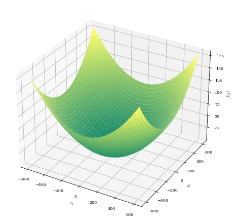
Bases: glompo.benchmark_fncs.BaseTestCase

Implementation of the Griewank optimization test function [b].

\[f(x) = \sum_{i=1}^d \frac{x_i^2}{4000} - \prod_{i=1}^d \cos\left(\frac{x_i}{\sqrt{i}}\right) + 1\]

Recommended bounds: \(x_i \in [-600, 600]\)

Global minimum: \(f(0, 0, ..., 0) = 0\)

class glompo.benchmark_fncs.Langermann(*args, shift_positive: bool = False, delay: float = 0)

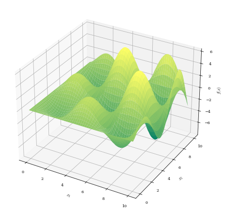
Bases: glompo.benchmark_fncs.BaseTestCase

When called returns evaluations of the Langermann function [a] [b].

\[\begin{split}f(x) & = & - \sum_{i=1}^5 \frac{c_i\cos\left(\pi\left[(x_1-a_i)^2 + (x_2-b_i)^2\right]\right)} {\exp\left(\frac{(x_1-a_i)^2 + (x_2-b_i)^2}{\pi}\right)}\\ \mathbf{a} & = & \{3, 5, 2, 1, 7\}\\ \mathbf{b} & = & \{5, 2, 1, 4, 9\}\\ \mathbf{c} & = & \{1, 2, 5, 2, 3\}\\\end{split}\]

Recommended bounds: \(x_1, x_2 \in [0, 10]\)

Global minimum: \(f(2.00299219, 1.006096) = -5.1621259\)

Parameters:shift_positive – Shifts the entire function such that the global minimum falls at ~0.

class glompo.benchmark_fncs.LennardJones(atoms: int, dims: int, eps: float = 1, sigma: float = 1, *, delay=None)

Bases: glompo.benchmark_fncs.BaseTestCase

Lennard-Jones energy potential function. Designed to predict the energy for clusters of atoms, this potential energy surface is characterized by steep cliffs, infinite values, and degenerate local and global minima.

The input vector \(\mathbf{x}\) is reshaped into an \(N \times d\) array (\(X\)) of \(d\)-dimensional Cartesian coordinates for \(N\) particles.

\[f(X) = 4\epsilon\sum_{i<j}{\left[\left(\frac{\sigma}{r_{ij}}\right)^{12} - \left(\frac{\sigma}{r_{ij}}\right)^6\right]}\]

where \(\epsilon\) and \(\sigma\) are parameters and \(r_{ij}\) is the Euclidean distance between particles \(i\) and \(j\).

Recommended bounds: \(x_i \in [-2^{-1/6}\sigma\sqrt[3]{\frac{\pi}{3N}}, 2^{-1/6}\sigma\sqrt[3]{\frac{\pi}{3N}}]\)

Global minimum: Estimated from \(N\) and \(d\)

Parameters:

• atoms – The number of particles (\(N\)).
• dims – The number of Cartesian spatial dimensions (\(d\)).
• eps – The magnitude parameter (\(\epsilon\)).
• sigma – The shape parameter (\(\sigma\)).

dims

The number of adjustable parameters in the optimization problem is \(Nd\).

Notes

The x parameter for the call method may be a \(Nd\) length vector or a \(N \times d\) array.

jacobian(x: Sequence[float]) → numpy.ndarray

Returns the gradient (first derivative) of the function in all directions, calculated analytically. :param x: Vector in parameter space where the function will be evaluated.

Returns:Vector of derivatives for each dimension in x. Return type:numpy.ndarray

class glompo.benchmark_fncs.Levy(dims: int, *, delay: float = 0)

Bases: glompo.benchmark_fncs.BaseTestCase

Implementation of the Levy optimization test function [b].

\[\begin{split}f(x) & = & \sin^2(\pi w_1) + \sum^{d-1}_{i=1}\left(w_i-1\right)^2\left[1+10\sin^2\left(\pi w_i +1 \right)\right] + \left(w_d-1\right)^2\left[1+\sin^2\left(2\pi w_d\right)\right] \\ w_i & = & 1 + \frac{x_i - 1}{4}\end{split}\]

Recommended bounds: \(x_i \in [-10, 10]\)

Global minimum: \(f(1, 1, ..., 1) = 0\)

class glompo.benchmark_fncs.Michalewicz(dims: int = 2, m: float = 10, *, delay: float = 0)

Bases: glompo.benchmark_fncs.BaseTestCase

Implementation of the Michalewicz optimization test function [b].

\[f(x) = - \sum^d_{i=1}\sin(x_i)\sin^{2m}\left(\frac{ix_i^2}{\pi}\right)\]

Recommended bounds: \(x_i \in [0, \pi]\)

Global minimum:

\[\begin{split}f(x) = \begin{cases} -1.8013 & \text{if} & d=2 \\ -4.687 & \text{if} & d=5 \\ -9.66 & \text{if} & d=10 \\ \end{cases}\end{split}\]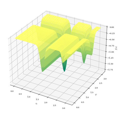

Parameters:m – Parametrization of the function. Lower values make the valleys more informative at pointing to the minimum. High values (\(\pm10\)) create a needle-in-a-haystack function where there is no information pointing to the minimum.

class glompo.benchmark_fncs.Qing(dims: int, *, delay: float = 0)

Bases: glompo.benchmark_fncs.BaseTestCase

Implementation of the Qing optimization test function [a].

\[f(x) = \sum^d_{i=1} (x_i^2-i)^2\]

Recommended bounds: \(x_i \in [-500, 500]\)

Global minimum: \(f(\sqrt{1}, \sqrt{2}, ..., \sqrt{n}) = 0\)

class glompo.benchmark_fncs.Rana(dims: int, *, delay: float = 0)

Bases: glompo.benchmark_fncs.BaseTestCase

Implementation of the Rana optimization test function [a].

\[\begin{split}f(x) = \sum^d_{i=1}\left[x_i\sin\left(\sqrt{\left|x_1-x_i+1\right|}\right) \cos\left(\sqrt{\left|x_1+x_i+1\right|}\right)\\ + (x_1+1)\sin\left(\sqrt{\left|x_1+x_i+1\right|}\right) \cos\left(\sqrt{\left|x_1-x_i+1\right|}\right) \right]\end{split}\]

Recommended bounds: \(x_i \in [-500.000001, 500.000001]\)

Global minimum: \(f(-500, -500, ..., -500) = -928.5478\)

class glompo.benchmark_fncs.Rastrigin(dims: int, *, delay: float = 0)

Bases: glompo.benchmark_fncs.BaseTestCase

Implementation of the Rastrigin optimization test function [b].

\[f(x) = 10d + \sum^d_{i=1} \left[x_i^2-10\cos(2\pi x_i)\right]\]

Recommended bounds: \(x_i \in [-5.12, 5.12]\)

Global minimum: \(f(0, 0, ..., 0) = 0\)

class glompo.benchmark_fncs.Rosenbrock(dims: int, *, delay: float = 0)

Bases: glompo.benchmark_fncs.BaseTestCase

Implementation of the Rosenbrock optimization test function [b].

\[f(x) = \sum^{d-1}_{i=1}\left[100(x_{i+1}-x_i^2)^2+(x_i-1)^2\right]\]

Recommended bounds: \(x_i \in [-2.048, 2.048]\)

Global minimum: \(f(1, 1, ..., 1) = 0\)

class glompo.benchmark_fncs.Schwefel(dims: int = 2, *, shift_positive: bool = False, delay: float = 0)

Bases: glompo.benchmark_fncs.BaseTestCase

Implementation of the Schwefel optimization test function [b].

\[f(x) = 418.9829d - \sum^d_{i=1} x_i\sin\left(\sqrt{|x_i|}\right)\]

Recommended bounds: \(x_i \in [-500, 500]\)

Global minimum: \(f(420.9687, 420.9687, ..., 420.9687) = -418.9829d\)

Parameters:shift_positive – Shifts the entire function such that the global minimum falls at ~0.

class glompo.benchmark_fncs.Shekel(dims: int = 2, m: int = 10, *, shift_positive: bool = False, delay: float = 0)

Bases: glompo.benchmark_fncs.BaseTestCase

Implementation of the Shekel optimization test function [b].

\[f(x) = - \sum^m_{i=1}\left(\sum^d_{j=1} (x_j - C_{ji})^2 + \beta_i\right)^{-1}\]

Recommended bounds: \(x_i \in [-32.768, 32.768]\)

Global minimum: \(f(4, 4, 4, 4) =~ -10\)

Parameters:

• m – Number of minima. Global minimum certified for m=5,7 and 10.
• shift_positive – Shifts the entire function such that the function is strictly positive. Since this is variable for this function the adjustment is +12 and thus the global minimum will not necessarily fall at zero.

class glompo.benchmark_fncs.Shubert(dims: int = 2, style: int = 1, *, shift_positive: bool = False, delay: float = 0)

Bases: glompo.benchmark_fncs.BaseTestCase

Implementation of the Shubert Type-I, Type-III and Type-IV optimization test functions [a].

\[\begin{split}f_I(x) & = & \sum^2_{i=1}\sum^5_{j=1} j \cos\left[(j+1)x_i+j\right]\\ f_{III}(x) & = & \sum^5_{i=1}\sum^5_{j=1} j \sin\left[(j+1)x_i+j\right]\\ f_{IV}(x) & = & \sum^5_{i=1}\sum^5_{j=1} j \cos\left[(j+1)x_i+j\right]\\\end{split}\]

Recommended bounds: \(x_i \in [-10, 10]\)

Parameters:

• style – Selection between the Shubert01, Shubert03 & Shubert04 functions. Each more oscillatory than the previous.
• shift_positive – Shifts the entire function such that the global minimum falls at 0.

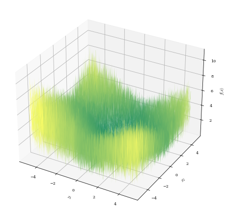
class glompo.benchmark_fncs.Stochastic(dims: int, *, delay: float = 0)

Bases: glompo.benchmark_fncs.BaseTestCase

Implementation of the Stochastic optimization test function [a].

\[\begin{split}f(x) & = & \sum^d_{i=1} \epsilon_i\left|x_i-\frac{1}{i}\right| \\ \epsilon_i & = & \mathcal{U}_{[0, 1]}\end{split}\]

Recommended bounds: \(x_i \in [-5, 5]\)

Global minimum: \(f(1/d, 1/d, ..., 1/d) = 0\)

class glompo.benchmark_fncs.StyblinskiTang(dims: int, *, delay: float = 0)

Bases: glompo.benchmark_fncs.BaseTestCase

Implementation of the Styblinski-Tang optimization test function [b].

\[f(x) = \frac{1}{2}\sum^d_{i=1}\left(x_i^4-16x_i^2+5x_i\right)\]

Recommended bounds: \(x_i \in [-500, 500]\)

Global minimum: \(f(-2.90, -2.90, ..., -2.90) = -39.16616570377 d\)

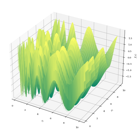
class glompo.benchmark_fncs.Trigonometric(dims: int, *, delay: float = 0)

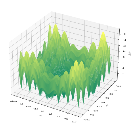
Bases: glompo.benchmark_fncs.BaseTestCase

Implementation of the Trigonometric Type-II optimization test function [a].

\[f(x) = 1 + \sum_{i=1}^d 8 \sin^2 \left[7(x_i-0.9)^2\right] + 6 \sin^2 \left[14(x_i-0.9)^2\right]+(x_i-0.9)^2\]

Recommended bounds: \(x_i \in [-500, 500]\)

Global minimum: \(f(0.9, 0.9, ..., 0.9) = 1\)

class glompo.benchmark_fncs.Vincent(dims: int, *, delay: float = 0)

Bases: glompo.benchmark_fncs.BaseTestCase

Implementation of the Vincent optimization test function [a].

\[f(x) = - \sum^d_{i=1} \sin\left(10\log(x)\right)\]

Recommended bounds: \(x_i \in [0.25, 10]\)

Global minimum: \(f(7.706, 7.706, ..., 7.706) = -d\)

class glompo.benchmark_fncs.ZeroSum(dims: int, *, delay: float = 0)

Bases: glompo.benchmark_fncs.BaseTestCase

Implementation of the ZeroSum optimization test function [a].

\[\begin{split}f(x) = \begin{cases} 0 & ext{if} \sum^n_{i=1} x_i = 0 \\ 1 + (10000|\sum^n_{i=1} x_i = 0|)^{0.5} & ext{otherwise} \end{cases}\end{split}\]

Recommended bounds: \(x_i \in [-10, 10]\)

Global minimum: \(f(x) = 0 ext{where} \sum^n_{i=1} x_i = 0\)